Gallery

Figures produced by the example apps in apps/, as captured by the apps regression baselines. Click any figure to enlarge.

Exercises

1_0_range_equation.py

Radar range equation exercises.

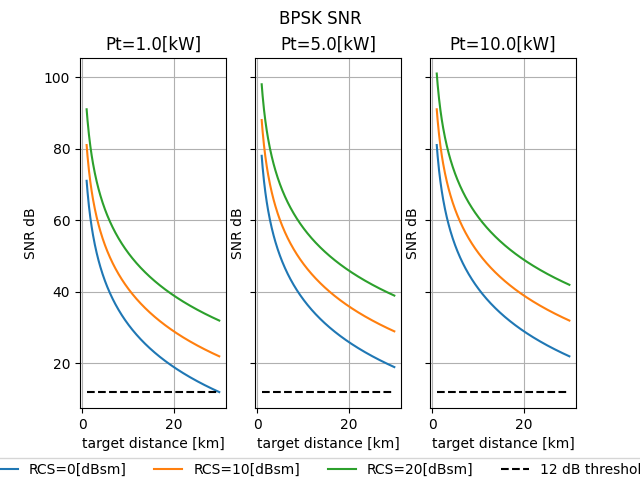
• Problem 1: Plot SNR vs range for a BPSK waveform across different transmit powers and target RCS values.
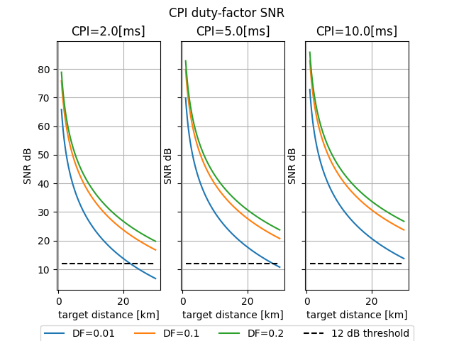
• Problem 2: Plot SNR vs range using the duty-factor form of the range equation across different CPI lengths and duty factors.
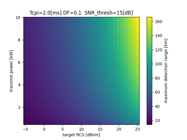
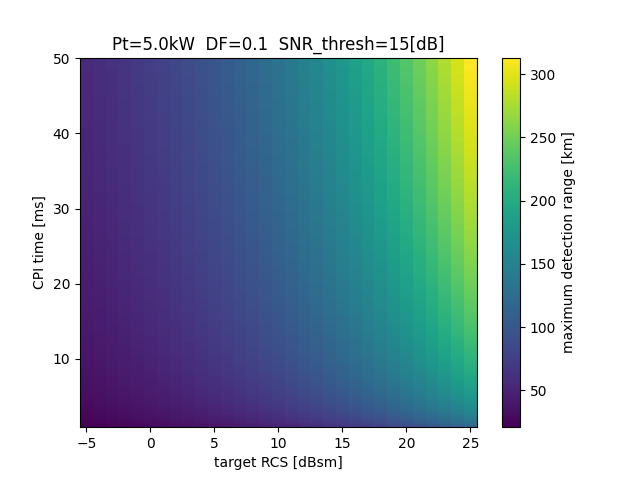
• Problem 3: Compute maximum detection range as a 2D function of (Tx power, RCS) and (CPI time, RCS), visualized as heatmaps.

2_0_pulse_doppler_radar.py

Pulse-Doppler radar ambiguity exercises.

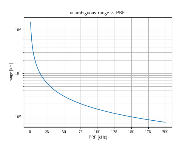
• Problem 1: Unambiguous range vs PRF.
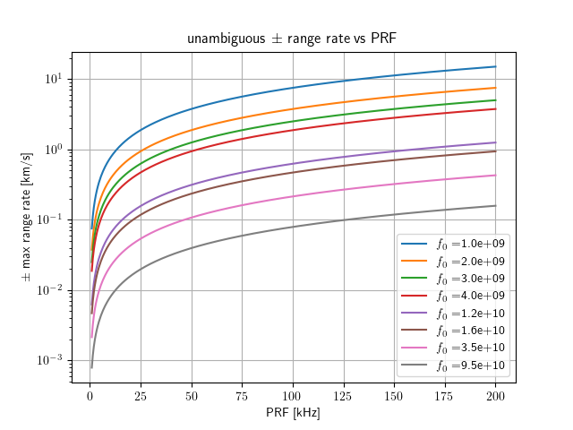
• Problem 2: Unambiguous range rate vs PRF for several carrier frequencies.
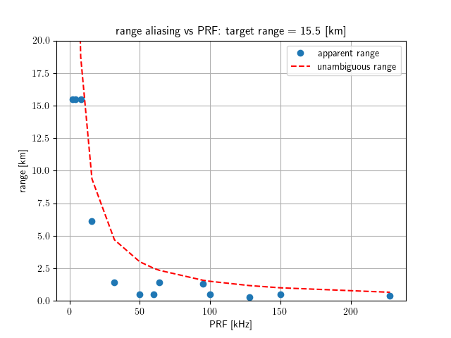
• Problem 3: Range aliasing — where a 15.5 km target appears at various PRFs.
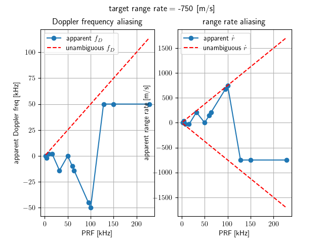
• Problem 4: Doppler and range-rate aliasing vs PRF.
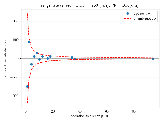
• Problem 5: Range-rate aliasing vs carrier frequency at fixed PRF.

3_1_waveforms_xcorrelation.py

Waveform cross-correlation exercises.

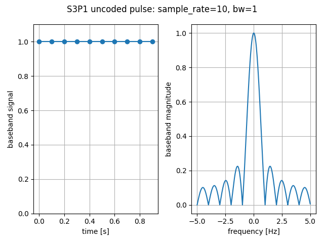
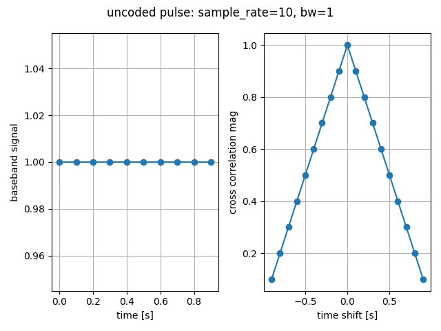
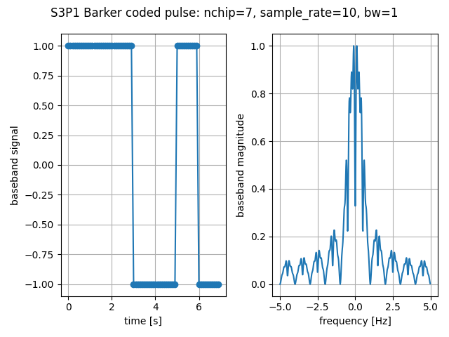
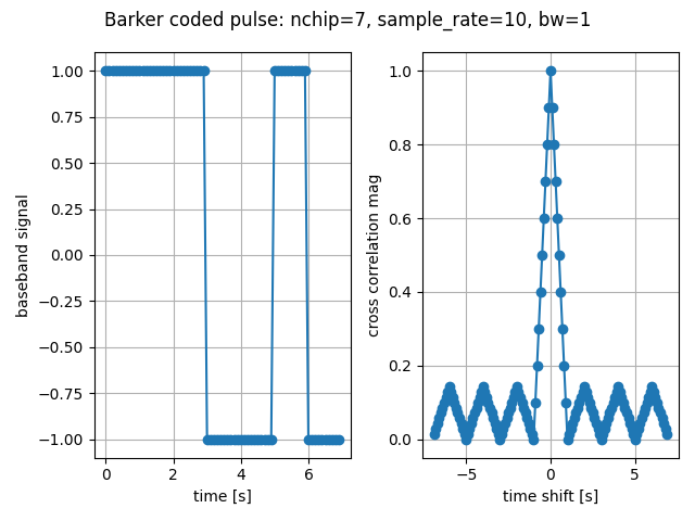
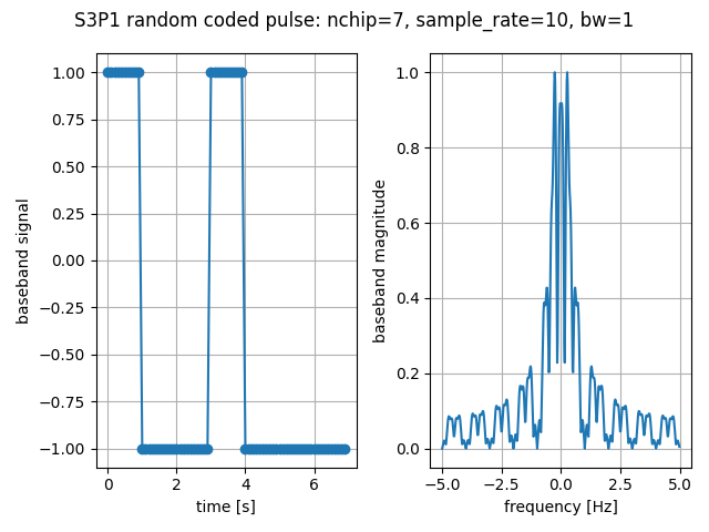
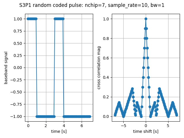
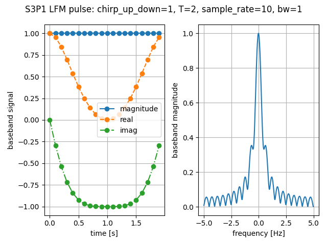
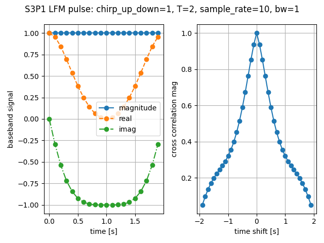
Generate uncoded, Barker-coded, random-coded, and LFM pulses, then visualize each pulse's time-domain shape, power spectral density, and auto-correlation.

Key takeaways:

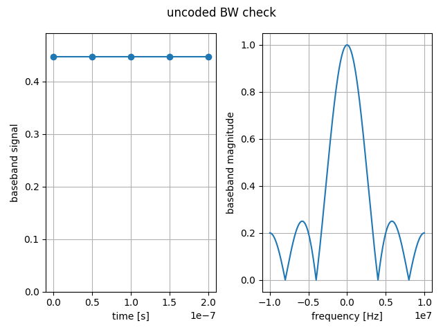
• BPSK bandwidth is set by the chip width (same as a single-chip pulse), but the PSD gets noisier with more chips.
• LFM spreads energy uniformly across the bandwidth.

3_2_barker_xcorrelation_sidelobes.py

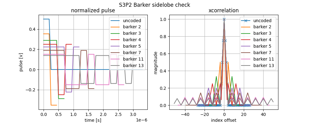
Barker code autocorrelation sidelobe comparison.

Compare the autocorrelation (matched-filter output) of an uncoded pulse to every standard Barker code length. Barker codes are prized because their autocorrelation sidelobes are at most 1/N of the peak, giving clean detection with minimal range ambiguity.

3_3_noisy_xcorrelations.py

Noisy cross-correlation (matched filter) exercises.

Show how a matched filter detects pulses buried in noise:

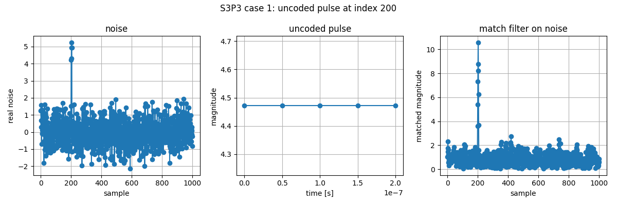
• Case 1: Single uncoded pulse at 20 dB SNR.
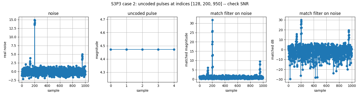
• Case 2: Three uncoded pulses at different SNRs (15, 30, 20 dB).
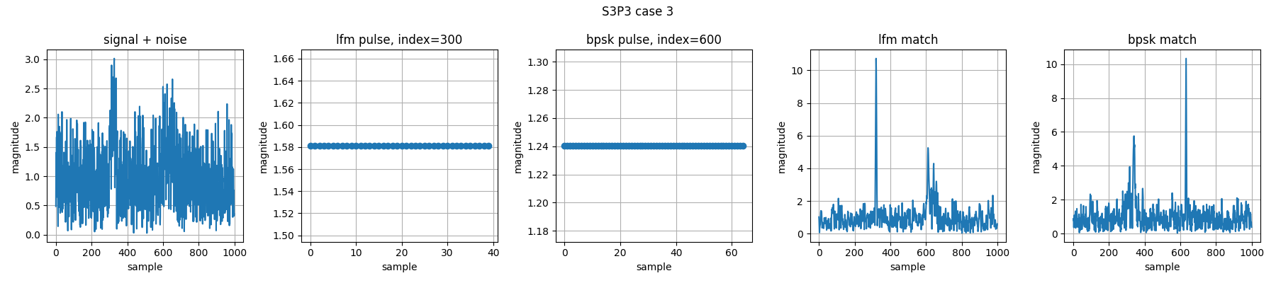
• Case 3: An LFM pulse and a Barker-13 BPSK pulse in the same noise — each matched filter responds only to its own waveform.

Key takeaway: the matched-filter peak appears at the center of the pulse (not the leading edge) and scales with the pulse's processing gain.

3_4_barker_vs_uncoded_ampAndWidth.py

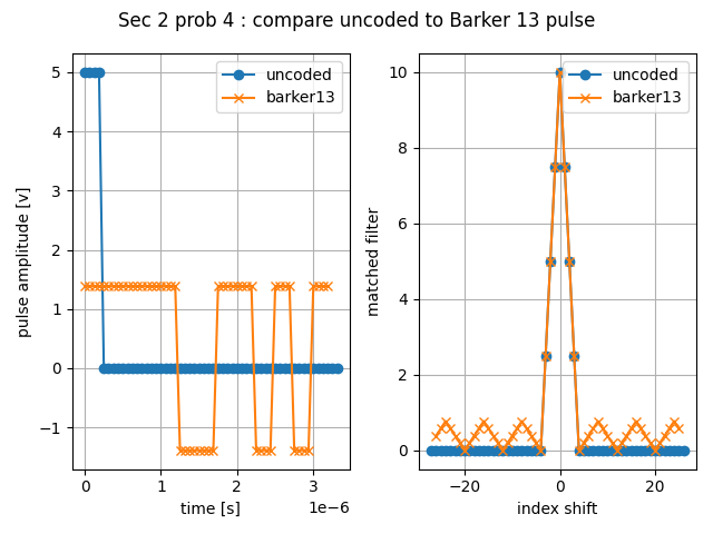
Compare Barker-13 vs uncoded pulse amplitude and matched-filter width.

Both pulses use the same chip bandwidth, so Barker-13 is 13x longer in time. Both are normalized to unit energy and scaled to the same SNR.

Key takeaways:

• Same energy spread over 13 chips at 1/sqrt(13) the amplitude, so the matched-filter peaks and -3 dB mainlobe widths come out identical.
• Barker reaches that energy at 13x lower peak power (easier on the transmitter), at the cost of autocorrelation sidelobes.
• The uncoded pulse has a clean triangular autocorrelation with none.

3_5_ambiguity_function.py

Ambiguity function exercises.

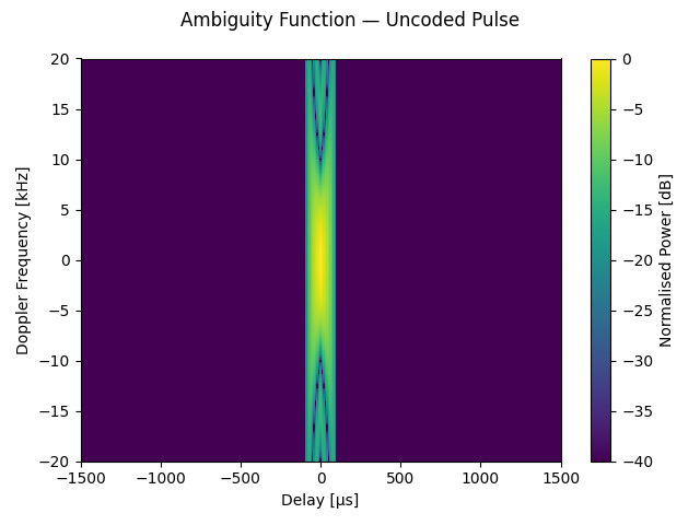
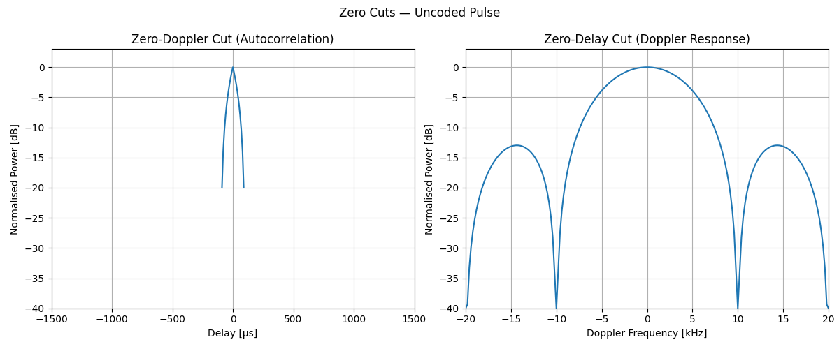
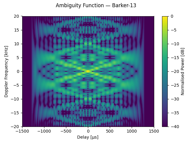
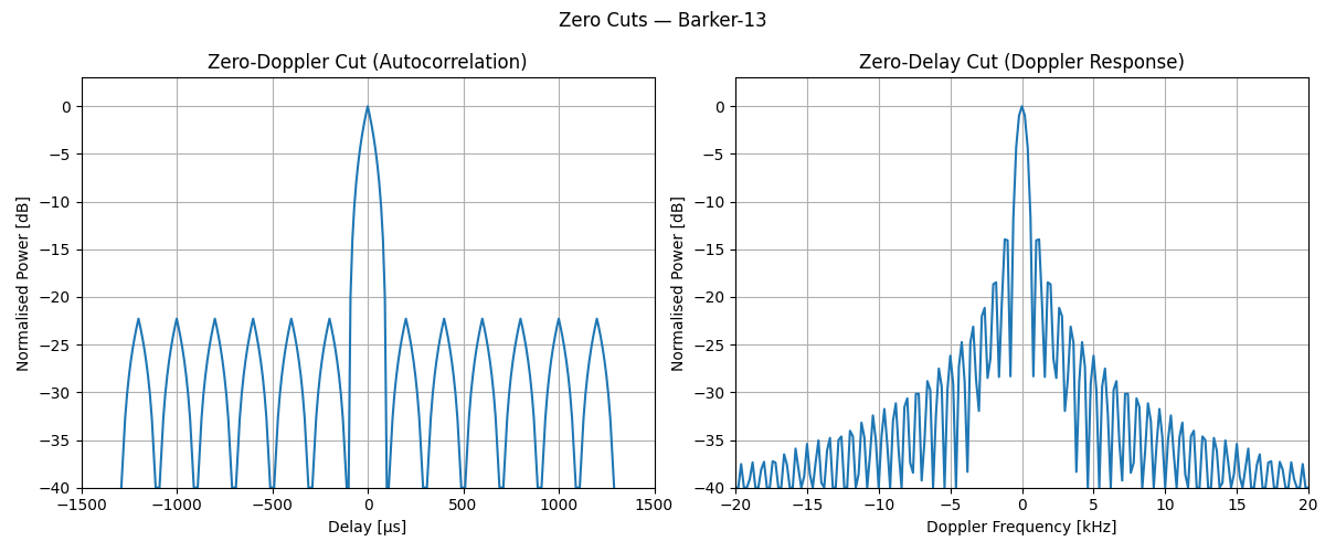
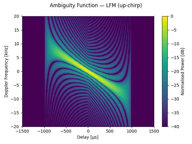
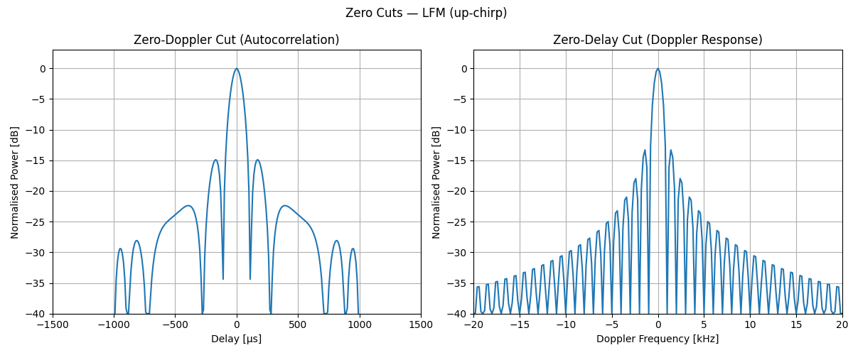
Compute and display the ambiguity function for three waveform types: uncoded, Barker-coded, and LFM. Plot each waveform's ambiguity surface and zero-delay / zero-Doppler cuts to illustrate the range-Doppler resolution tradeoffs.

Key takeaways:

• Uncoded pulse: triangular in delay (width set by the pulse length) and a sinc ridge in Doppler — a short pulse tolerates large Doppler shifts but resolves velocity poorly.
• Barker-coded pulse: same delay mainlobe width as a single chip but the surface approaches a "thumbtack" — energy is spread into low pedestal sidelobes across both delay and Doppler, sharpening joint resolution.
• LFM pulse: a diagonal ridge showing range-Doppler coupling. Narrow in both dimensions, but a target's apparent range shifts with its Doppler frequency.

4_1_datacube_process_test.py

Datacube processing test.

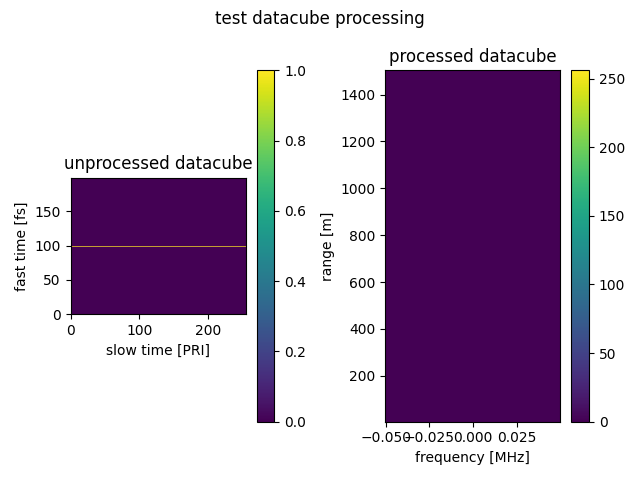
Build a raw RF datacube, inject a tone at a known range bin and Doppler frequency, then apply Doppler processing (FFT across slow time) to verify the signal appears in the correct range-Doppler cell.

The datacube has two axes:

• Fast time (rows): samples within a single PRI — maps to range.
• Slow time (columns): one sample per pulse — maps to Doppler frequency.

4_4_windowing_comparison.py

Window function comparison on a rectangular pulse.

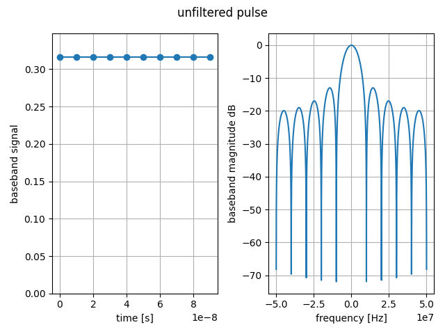
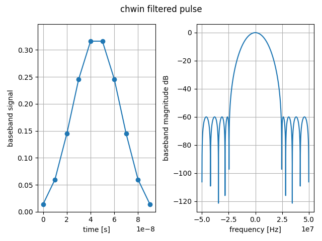
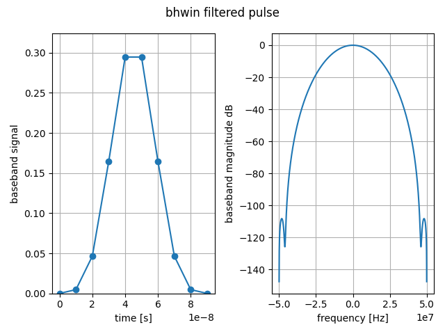
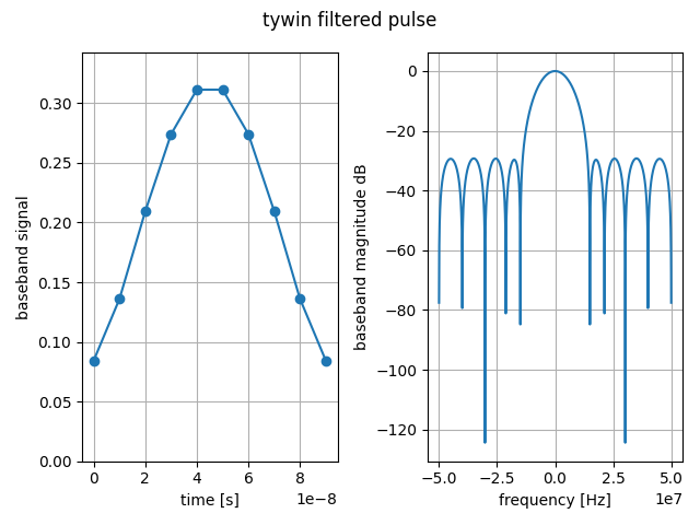
Apply Chebyshev, Blackman-Harris, and Taylor windows to an uncoded pulse and compare the resulting spectra. Windowing reduces spectral sidelobes at the cost of widening the mainlobe (lower range resolution).

Key takeaways:

• Unwindowed (rectangular): narrowest mainlobe, highest sidelobes (~-13 dB).
• Chebyshev: equi-ripple sidelobes at the specified level (60 dB here).
• Blackman-Harris: very low sidelobes, but widest mainlobe.
• Taylor: compromise — low near-in sidelobes with moderate mainlobe widening.

4_5_complex_tone.py

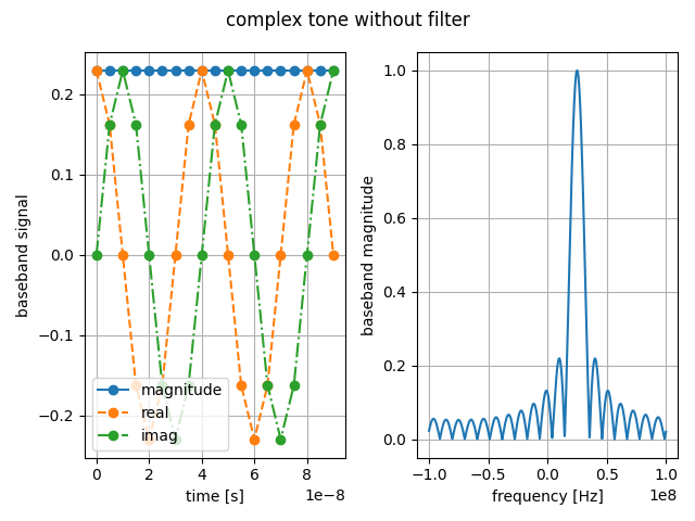
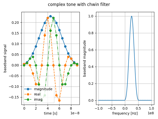
Complex tone windowing exercise.

Generate a complex tone (single-frequency sinusoid) and show how spectral leakage from the rectangular window is suppressed by applying a Chebyshev window before computing the spectrum.

5_0_stationary_rdm_snapshot.py

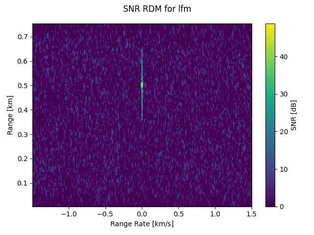
Stationary target RDM snapshot with SNR check.

Generate a range-Doppler map for a single stationary target (range_rate=0) using an LFM waveform and verify the SNR matches the range equation prediction.

Notes:

• The Matlab reference solution underestimates SNR because it omits the time-bandwidth product gain from pulse compression.
• Range walk-off is negligible here since the target is stationary.

6_1_detection_theory.py

Detection theory fundamentals.

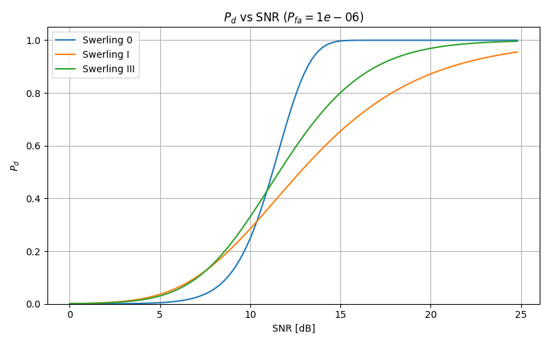
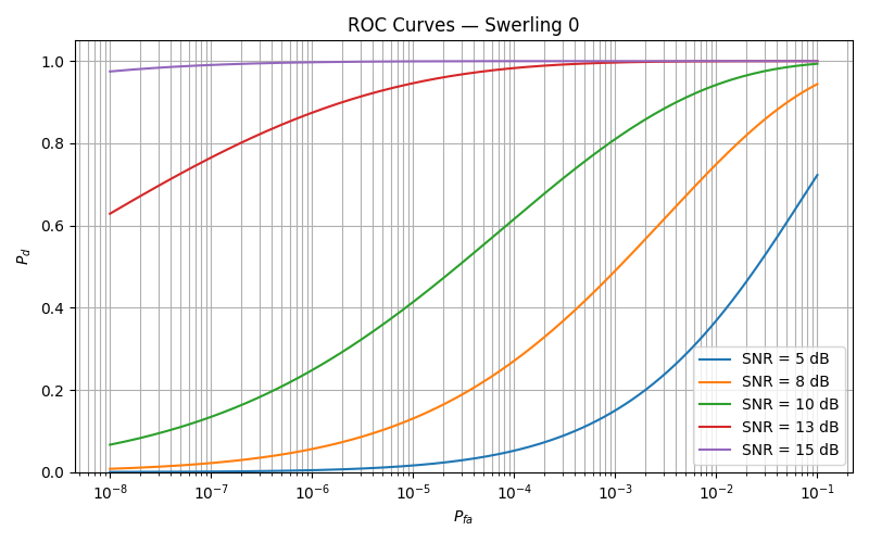
Demonstrate the relationship between SNR, probability of false alarm (Pfa), and probability of detection (Pd) for non-fluctuating and fluctuating targets.

Produces four figures:

1. Pd vs SNR for Swerling 0, I, and III at a fixed Pfa.
2. ROC curves (Pd vs Pfa) for Swerling 0 at several SNR values.
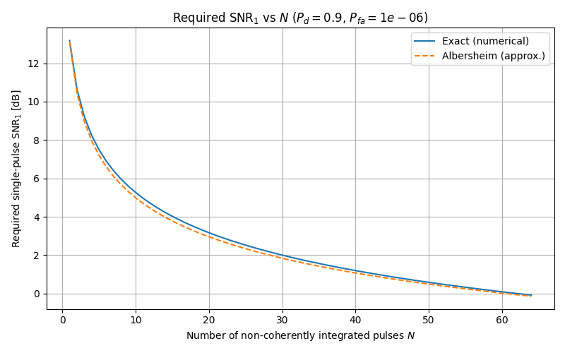
3. Required SNR vs number of non-coherently integrated pulses, comparing exact numerical results with Albersheim's approximation.
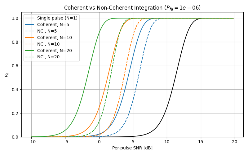
4. Pd vs per-pulse SNR comparing coherent integration and non-coherent integration of the same N pulses.

Key takeaways:

• A non-fluctuating target (Swerling 0) has the steepest Pd-vs-SNR curve. Fluctuating targets (Swerling I, III) require higher average SNR for the same Pd because the instantaneous RCS can be much lower than the average.
• Swerling III (4 DOF) performs better than Swerling I (2 DOF) because its RCS is less likely to fade to zero.
• Integrating N pulses either way beats a single pulse, but coherent integration gains the full factor of N in SNR while NCI gains less (roughly N^0.7-0.8 here). The NCI loss grows with N: about 1.3 dB at N=5 and 3 dB at N=20 for Pd = 0.9, Pfa = 1e-6.
• Albersheim's closed-form approximation tracks the exact numerical result to within a fraction of a dB over most of its stated validity range (0.1 <= Pd <= 0.9, 1e-7 <= Pfa <= 1e-3, 1 <= N <= 8096), degrading only toward the low-Pd / high-Pfa corner.

6_2_cfar_kernels.py

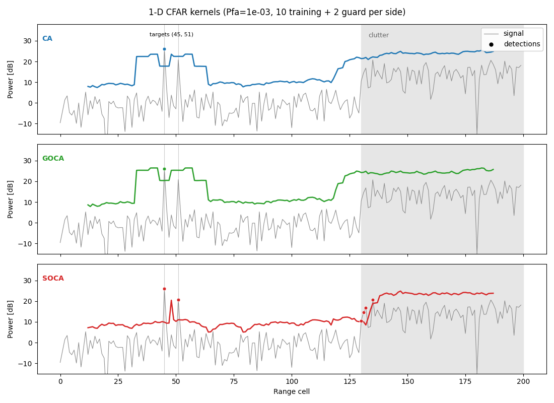
CFAR kernels in 1-D: how CA, GOCA, and SOCA differ.

The applied CFAR exercise (6_3) runs on a 2-D range-Doppler map, where the detection threshold is a surface you cannot see directly. Strip the problem down to a single range profile so the threshold is a line drawn on top of the signal, making the kernel arithmetic visible:

Each cell under test (CUT) estimates the local noise from N_TRAIN training cells on each side (a guard band around the CUT is excluded). The three kernels combine the leading and lagging halves differently:

CA    noise = mean(all 2*N_TRAIN training cells)
GOCA  noise = max(mean(leading half), mean(lagging half))
SOCA  noise = min(mean(leading half), mean(lagging half))

The threshold is alpha * noise, where noise is the training-cell power estimate and alpha is the multiplier that sets it high enough for a noise-only cell's exceedance probability to equal Pfa (exact for CA under exponential, square-law noise). This is the same CA multiplier used in cfar_2d; GOCA and SOCA reuse it as an approximation (their exact multipliers have no closed form), so their realised false-alarm rate drifts from Pfa.

The profile contains two features that expose the trade-offs:

1. Two closely-spaced targets, near enough that each sits in the other's training window.
2. A clutter edge — a step up in noise power.

Key takeaways:

• Target masking: the strong target inflates one half of the weaker target's window. CA averages it in and GOCA keys on that inflated half, raising the threshold until the weak target is MASKED. SOCA keys on the clean half and still detects it.
• Clutter edge: SOCA clings to the low (clear) side as the window crosses the edge, so its threshold lags and it fires false alarms just inside the clutter. GOCA keys on the high side and stays clean; CA ramps between.
• No kernel wins everywhere: SOCA resists mutual-target masking but is worst at clutter edges; GOCA is the reverse; CA is the compromise.

6_3_cfar_lfm_sidelobes.py

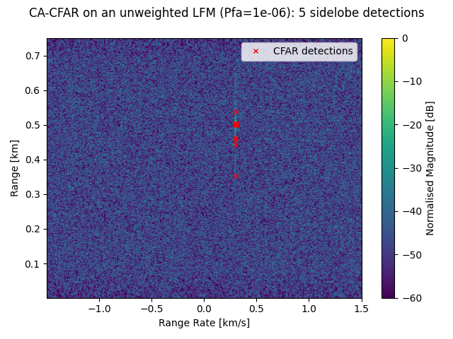
CA-CFAR on an unweighted LFM RDM: detections land on the range sidelobes.

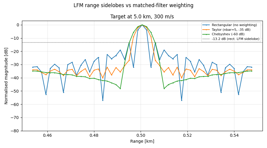
An LFM (chirp) pulse compresses to a sinc-like range response whose peak sidelobes sit only ~-13.2 dB below the mainlobe. CFAR sets its threshold from the local noise floor and knows nothing of pulse shape, so around a strong target it fires not just on the mainlobe but on the sidelobes too -- a column of spurious "targets" in range where there is really one.

This is the problem. Exercise 6_4 (LFM range windowing) is the fix, and 6_5 carries the fix into the CFAR-variant comparison.

6_4_lfm_range_windowing.py

LFM range-sidelobe suppression by matched-filter weighting.

The problem:

• An LFM (chirp) compresses to a sinc-like range response with peak sidelobes only ~-13.2 dB below the mainlobe.
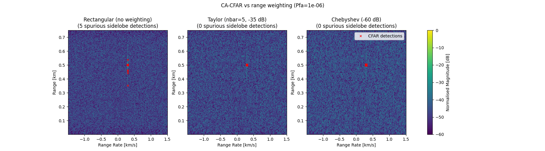
• CFAR thresholds off the local noise floor and knows nothing of pulse shape, so around a strong target it fires on those sidelobes -- a smear of spurious "targets" where there is really one.
• CFAR cannot fix this itself: a -13 dB sidelobe is a real power excess.

The fix (one stage earlier, in pulse compression): weight the matched-filter replica. An LFM's frequency is linear in time, so tapering the replica in time tapers the swept-spectrum edges -- the frequency weighting Richards uses for range-sidelobe control. Sidelobes drop below threshold; the cost is a broader mainlobe (coarser range resolution) and a small SNR loss.

Produces two figures:

• Fig 1: noiseless range point-spread (rectangular vs Taylor vs Chebyshev) — the -13.2 dB pedestal buried, the mainlobe widened.
• Fig 2: CA-CFAR on the noisy RDM — the spurious sidelobe detections vanish.

Printed per window: peak sidelobe level, -3 dB mainlobe width, weighting loss, CFAR detection count.

Reference: Richards, M. A., Fundamentals of Radar Signal Processing, 2nd ed., McGraw-Hill, 2014, Ch. 4 (Radar Waveforms) -- matched filter, LFM pulse compression, the ~-13.2 dB sidelobes, and their reduction by amplitude weighting with the attendant processing-gain loss. CFAR is Ch. 7.

6_5_cfar_detection.py

CFAR detection on a range-Doppler map (with LFM range weighting).

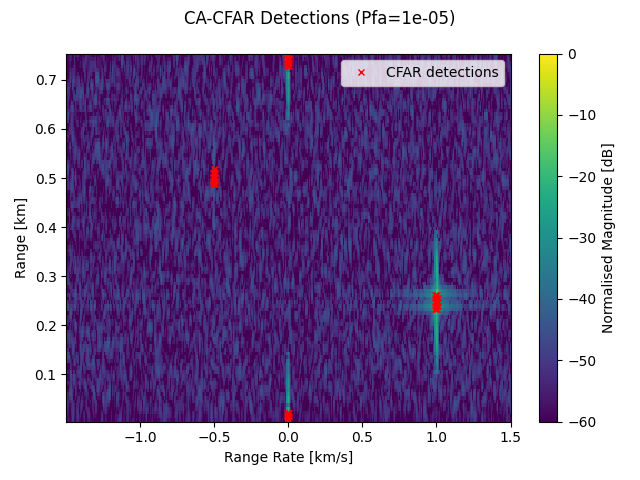
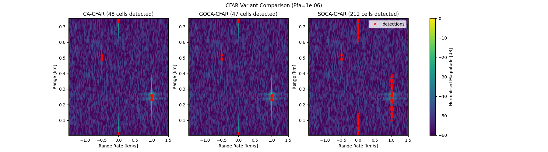
Generate an RDM with three targets at different ranges and velocities, then apply Cell-Averaging CFAR (CA-CFAR) to detect them. The matched filter is Taylor-weighted for range-sidelobe control (see exercise 6_4), so the LFM's ~-13.2 dB range sidelobes stay below the CFAR threshold and do not clutter the map with spurious detections -- isolating the behaviour of the CFAR variants themselves. The exercise produces four figures:

1. The raw RDM with noise floor and target peaks.
2. CA-CFAR detection markers overlaid on the RDM.
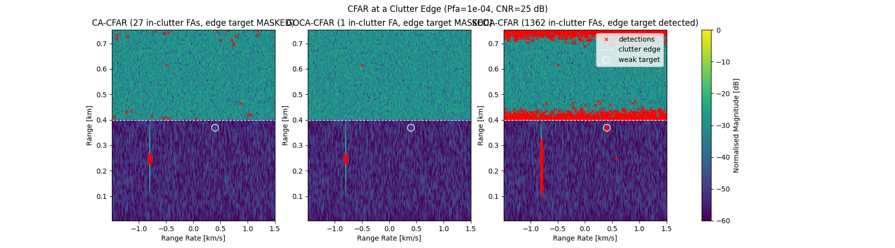
3. A comparison of CA-CFAR, GOCA-CFAR, and SOCA-CFAR on the same RDM.
4. A clutter-edge scene where the variants actually differ: GOCA suppresses the false alarms CA and SOCA fire along the edge, while SOCA detects a weak target near the edge that clutter in the training window masks from CA and GOCA.

Key takeaways:

• CFAR adapts the detection threshold to the local noise level, maintaining a constant false alarm rate without requiring a fixed threshold.
• Guard cells prevent signal energy from leaking into the noise estimate.
• In homogeneous noise the variants only shift the threshold (SOCA lowest, GOCA highest); their real differences appear at a clutter edge. Inside the clutter, a window straddling the edge drags the CA threshold down (false alarms; SOCA far worse), while GOCA keys on the clutter half and stays clean. Just outside the clutter, the same straddling inflates the CA and GOCA thresholds (masking weak targets), while SOCA keys on the clear half and still detects. CA is the compromise; no variant wins everywhere.

7_0_linear_array_studies.py

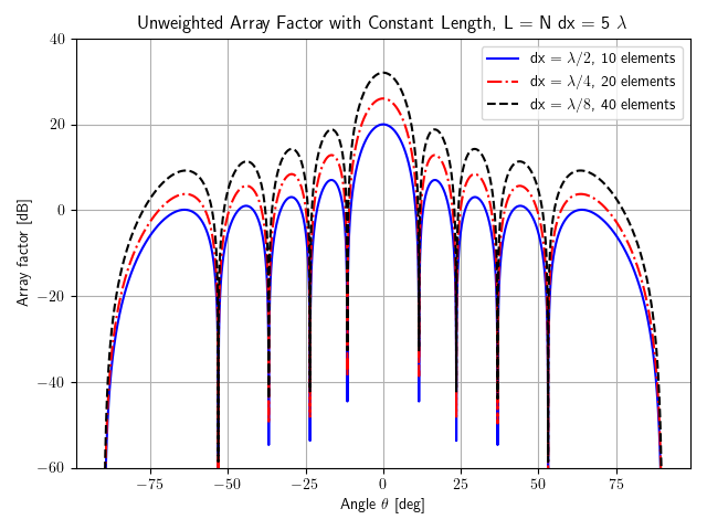
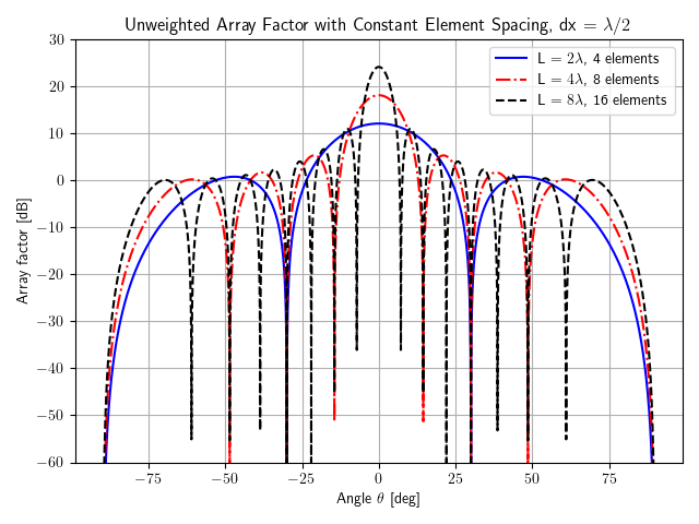
Uniform linear array (ULA) studies.

Background: each element receives the signal with a phase shift proportional to d*sin(theta)/lambda, where d is the element spacing.

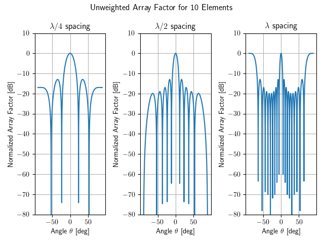
• Study 1 — constant length, varying element spacing: as long as dx <= lambda/2 (no grating lobes), the array-factor shape is set by the total length N*dx, not the element count. Adding elements only raises the peak (more coherent sum). Beamwidth scales as 0.886/(N*dx) radians, so equal N*dx means equal beamwidth.
• Study 2 — constant spacing (lambda/2), varying element count: a longer array gives a narrower mainlobe (higher angular resolution) — the Fourier-transform duality, like a longer time signal giving a narrower spectral peak.

7_1-3_linear_arrays_figs24_28.py

Recreate textbook figures 24-28 for uniform linear arrays.

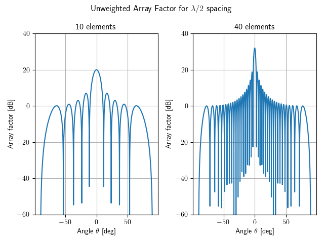
• Figure 24: number of elements vs the array factor (lambda/2 spacing).
• Figure 25: element spacing vs the array factor (10 elements); spacing > lambda/2 introduces grating lobes.
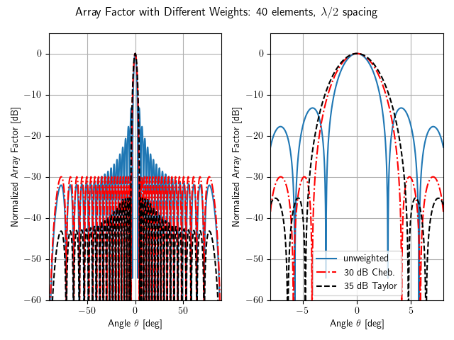
• Figure 27: weighted array factors (Chebyshev, Taylor) vs unweighted — weighting suppresses sidelobes at the cost of mainlobe width.
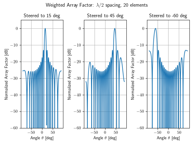
• Figure 28: beam steering to 15, 45, and -60 degrees — steering broadens the beam and lowers peak gain at large angles.

Scaling note vs the reference document:

• These figures plot the voltage array factor in dB, 20*log10|AF|, peaking at 20*log10(N). The reference plots 10*log10 quantities (power gain, dBi), so its unnormalized peaks sit at half our dB values — different (voltage vs power) conventions, not a bug.
• Figures 27 and 28 are normalized to their peaks, so the convention cancels and they match the document directly.

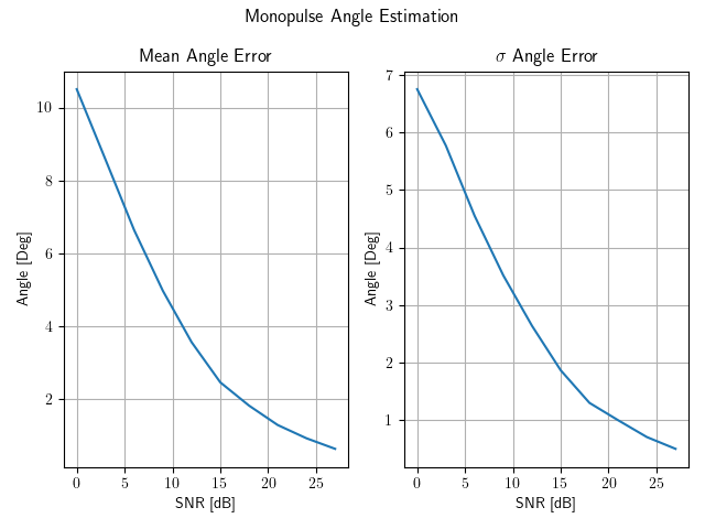
7_5_monopulse_snr_test.py

Monopulse angle estimation accuracy vs SNR.

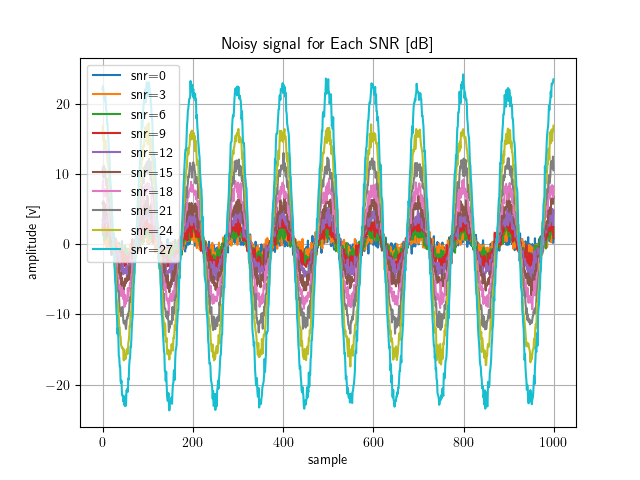
Simulate a two-element array receiving a signal from a known angle, add noise at varying SNR levels, and measure how accurately the monopulse ratio estimates the target angle.

Monopulse works by comparing the signals at two array elements (sum and difference channels). The ratio of difference to sum gives an angle estimate that is independent of signal amplitude.

Key takeaways:

• Estimation accuracy improves dramatically with SNR.
• Accuracy also depends on the true target angle (closer to boresight is better).

7_5_monopulse_snr_test_freq.py

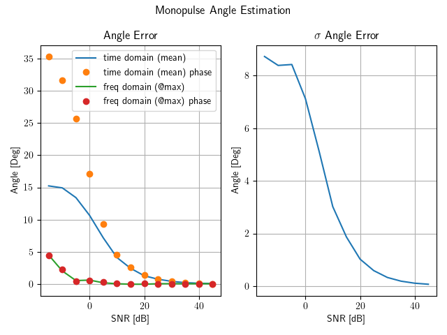
Monopulse angle estimation: time-domain vs frequency-domain comparison.

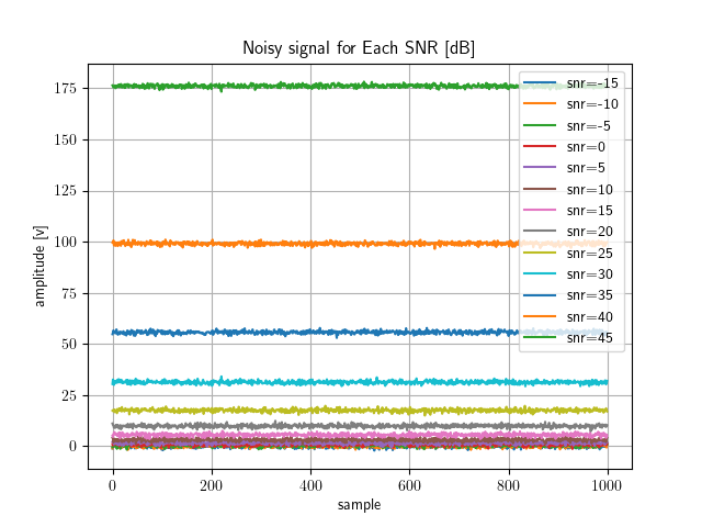
Extend the basic monopulse SNR test (7_5) to show that monopulse angle estimation works identically in both domains. Compare four methods:

1. Time-domain monopulse ratio (sum/difference of element signals)
2. Time-domain phase-only estimate (only valid at baseband, not RF passband)
3. Frequency-domain monopulse ratio (applied at the peak FFT bin)
4. Frequency-domain phase-only estimate (survives at RF: the peak bin demodulates the tone)

There is no pulse train here: the record is a single dwell of N complex samples of one tone. "Coherent integration" means summing those N samples, which gives ~10*log10(N) of SNR gain. Both domains do exactly that same sum before forming the ratio -- the time domain adds the samples directly (at RF, after demodulating the tone), and the frequency domain reads the peak FFT bin, which is that identical sum written in the frequency domain (bit-for-bit equal when unwindowed). Errors are averaged over Monte Carlo noise trials at each SNR.

Key takeaways:

• The monopulse ratio gives the same accuracy in time and frequency domains, because both apply the one coherent sum over the N-sample dwell (the time-domain sum equals the peak FFT bin).
• The naive phase-only estimate reads the angle straight from the inter-element phase difference. It works at baseband, but the time-domain version fails at RF passband (summing the spinning carrier destroys the signal); the frequency-domain version survives because reading the peak bin demodulates the tone.

7_6_phase_center_location.py

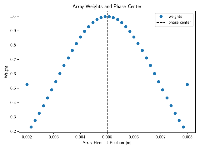
Array phase center calculation.

Compute the phase center of a weighted linear array. The phase center is the weighted centroid of the element positions — it tells you the effective "electrical center" of the array, which matters for monopulse and interferometric processing.

For a symmetric, uniformly-weighted array the phase center is at the geometric center. Asymmetric weighting shifts it toward the heavier-weighted elements.

Note: the reference document has an error in the phase center equation — it omits the normalization by the sum of weights.

7_7_sub_array_sum_diff.py

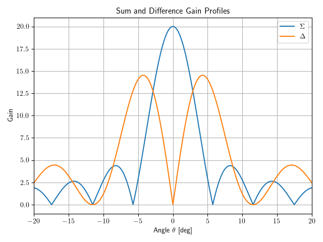
Sub-array sum and difference beam patterns for monopulse.

Split a 20-element ULA into left and right halves (sub-arrays), compute each sub-array's gain pattern, then form the sum (Sigma) and difference (Delta) beams.

The sum beam has maximum gain at boresight — used for detection and tracking. The difference beam has a null at boresight — used for angle estimation. The monopulse ratio (Delta/Sigma) gives a steep, monotonic curve near boresight that maps directly to target angle.

7_8_monopulse_tgt_doppler_cell.py

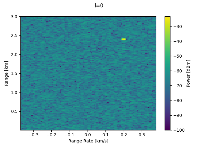
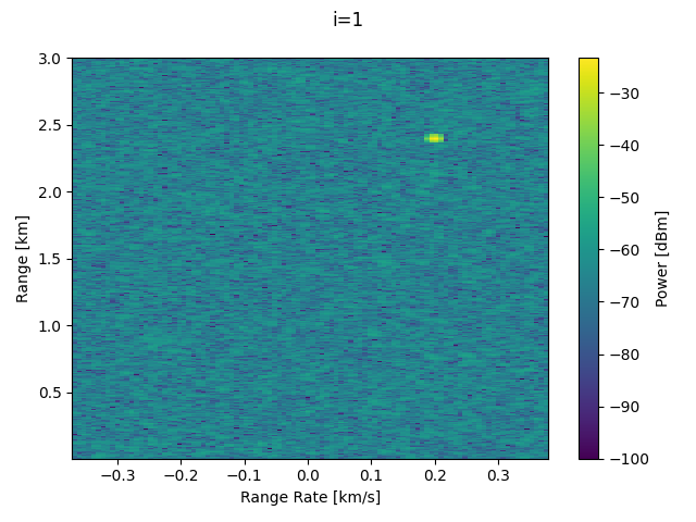
Monopulse angle estimation on a range-Doppler map.

Demonstrate that monopulse processing can be applied after Doppler processing (FFT along slow time). The workflow:

1. Define a two-element array and compute steering vectors for the target angle.
2. Generate a separate RDM for each array element (same noise seed so the noise realization is identical — only the signal phase differs).
3. Apply monopulse at the peak cell of the RDMs to estimate the target angle.

This validates that the inter-element phase relationship is preserved through matched filtering and Doppler processing.

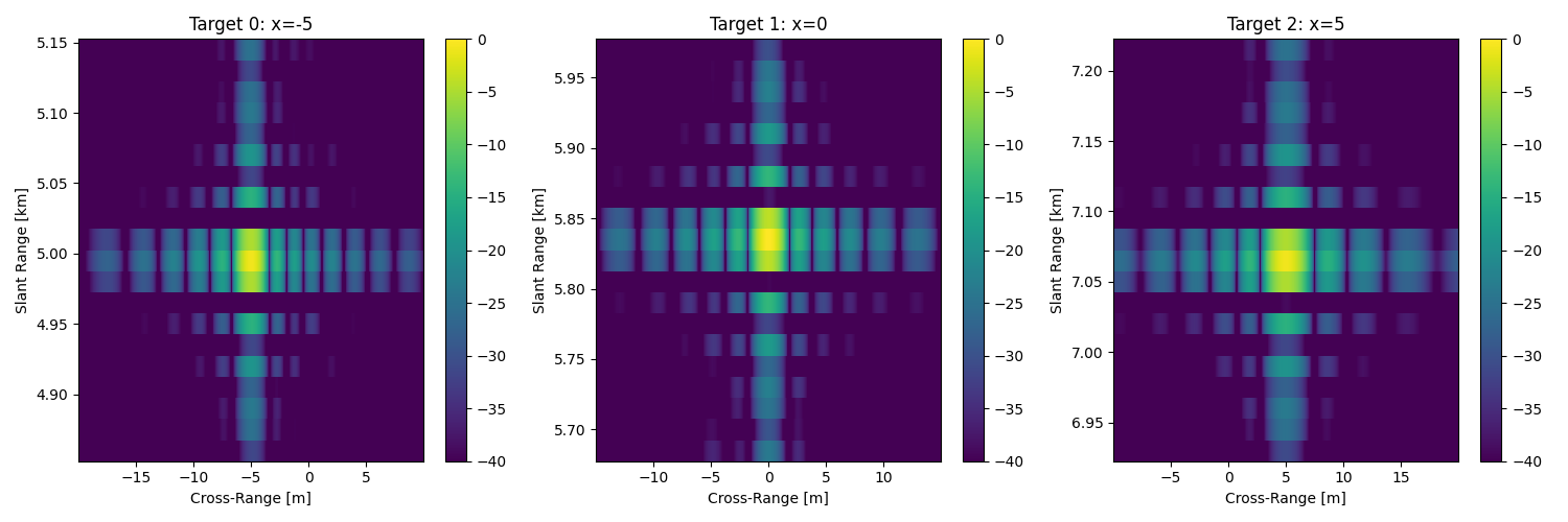
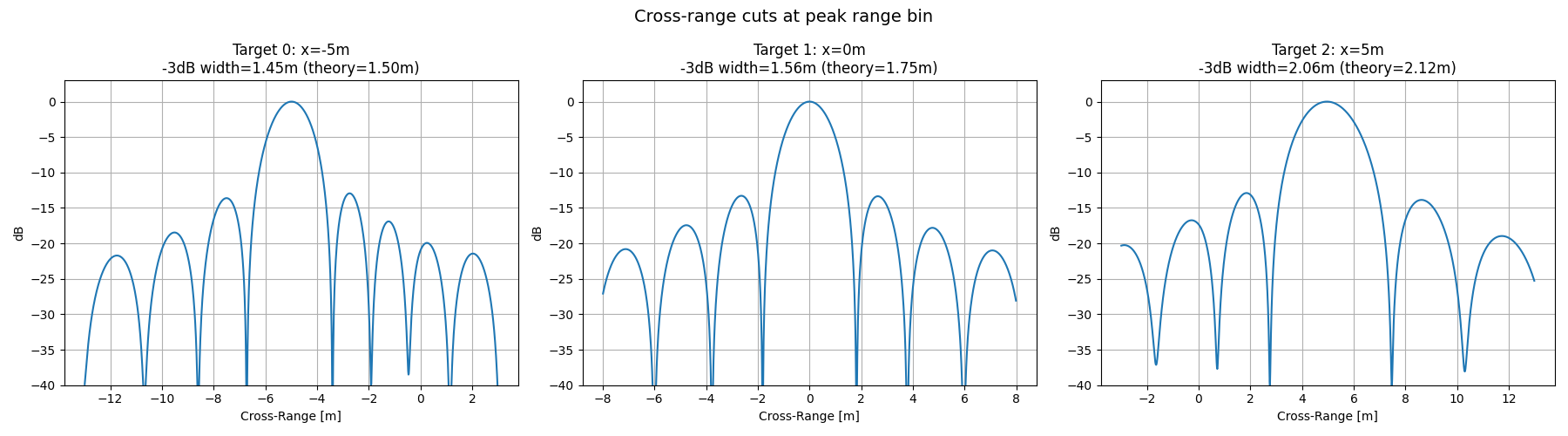
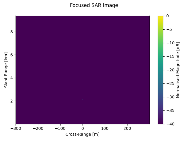
8_1_stripmap_sar_validation.py

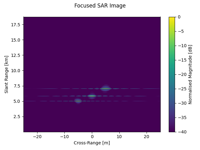
Validate an un-windowed stripmap SAR example.

Generates three figures:

1. Full SAR image from sar.gen.
2. ±150 m range, ±15 m cross-range zoom around each target — expect sinc-like patterns along both the range and cross-range axes.
3. Cross-range cuts through the peak range bin of each target — compares the measured -3 dB mainlobe width to the theoretical resolution λR/(2L) for an un-windowed SAR image.

8_3_stripmap_vs_spotlight.py

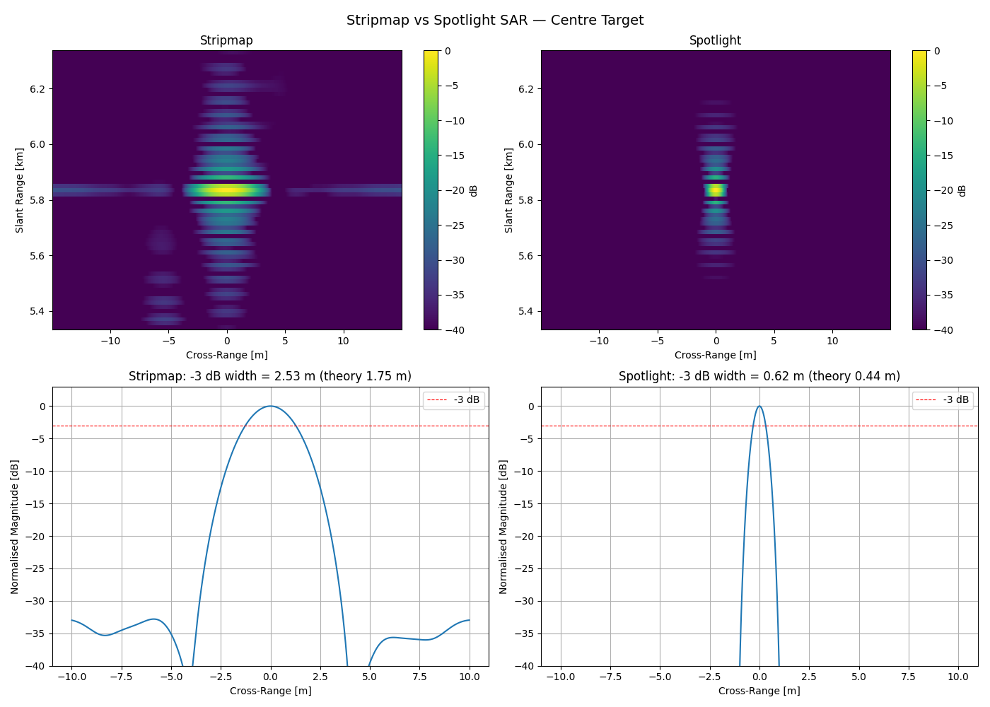
Side-by-side comparison of stripmap and spotlight SAR.

Run both modes on the same scene and plot:

• Top row: focused SAR images (stripmap vs spotlight).
• Bottom row: cross-range cuts through the centre target, with -3 dB width annotations.

The spotlight aperture is 4× longer, yielding ~4× finer cross-range resolution.

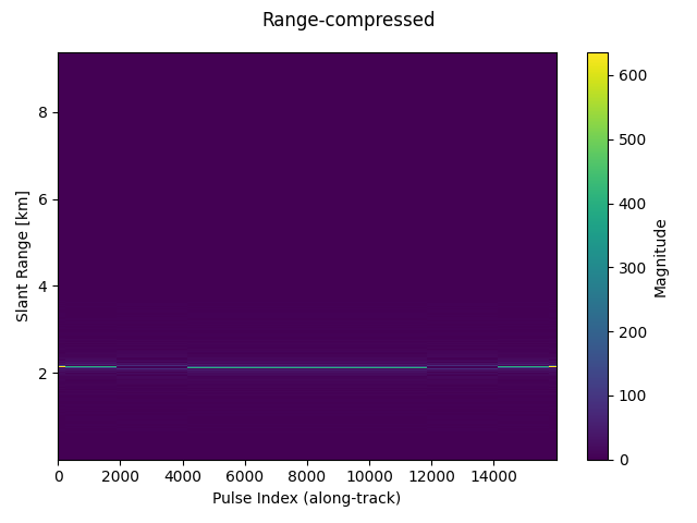
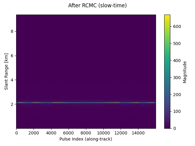
8_4_rcmc_demonstration.py

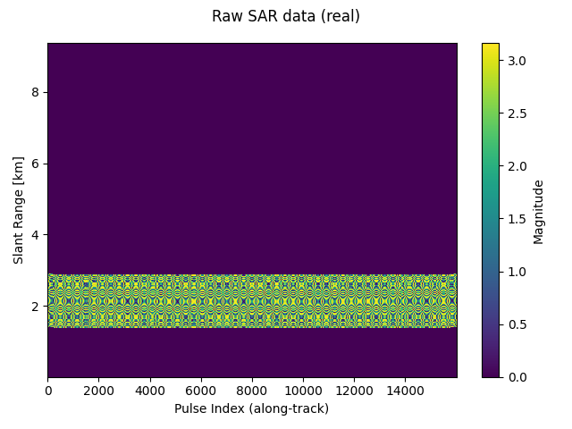
Demonstrate Range Cell Migration Correction (RCMC).

Run sar.gen twice on a long-aperture / close-range collection whose peak range migration spans multiple range cells, then print the azimuth peak position vs range bin offset for each. Without RCMC the azimuth peak tilts across neighbouring range bins (the RCM signature); with RCMC it sits at a constant cross-range position.

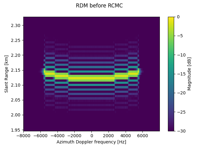
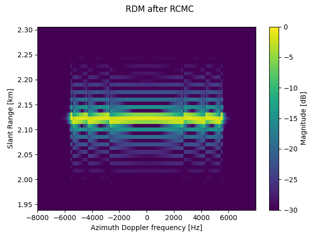
The first rcmc=True run is also called with debug=True so the range-Doppler map is plotted before and after the correction. In the "before" panel each target traces a curved hyperbola across Doppler frequency; in the "after" panel those curves collapse to straight horizontal lines at each target's closest-approach range.

8_5_rcmc_synthetic_validation.py

Validate RCMC against the closed-form migration formula.

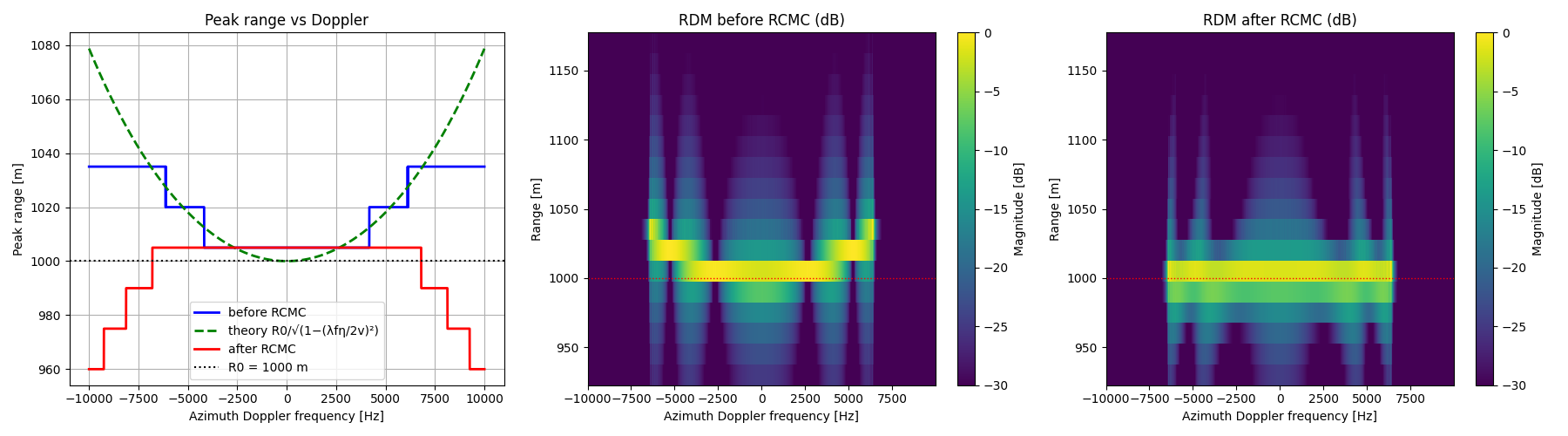
Bypass sar.gen and synthesise a perfectly range-compressed signal: at each pulse eta, the target's energy is a unit sinc lobe centred on the analytic slant range R(eta) = sqrt(R0^2 + v^2 eta^2), modulated by the two-way carrier phase exp(-j 4 pi R(eta) / lambda).

In the range-Doppler domain (azimuth FFT applied) the energy follows the exact parabolic curve

R(f_eta) = R0 / sqrt(1 - (lambda * f_eta / (2 v))^2)

which RCMC should straighten to a horizontal line at R0. The figure overlays the measured trajectory before and after RCMC on this theory curve, and shows the range-Doppler map in dB before and after correction.

RDMs

jammer_offset.py

Jammer with range and Doppler offset.

Demonstrate a DRFM jammer that retransmits with offsets in both range and Doppler, pulling the apparent target away from its true position.

EaPlatform offset parameters:

• range_offset: shifts the jammer response in range [m] (negative = closer).
• rdot_offset: shifts the VBM noise center in Doppler [m/s].
• rdot_delta: width of the VBM Doppler spread [m/s].
• delay: additional time delay before retransmission [s].

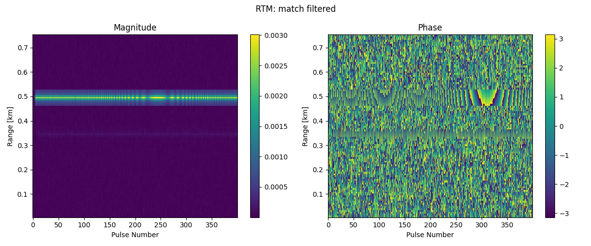
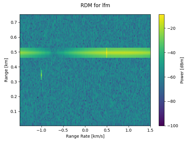
kitchen_sink.py

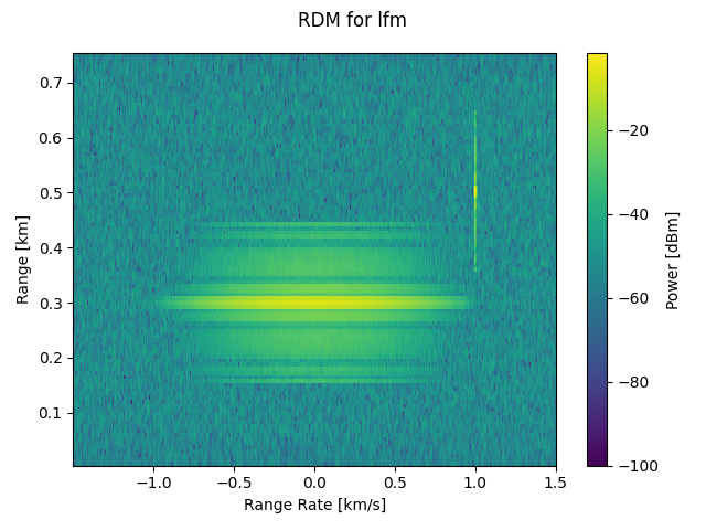
Kitchen-sink example: demonstrates all major RDM generation options.

This script shows how to combine:

• Different waveform types (uncoded, Barker, random-coded, LFM)
• A passive skin return (no jammer)
• A DRFM jammer return with range/Doppler offsets and a steering vector
• Debug and plotting options for rdm.gen()

The last waveform assignment wins, so uncomment the one you want to try.

readme_example.py

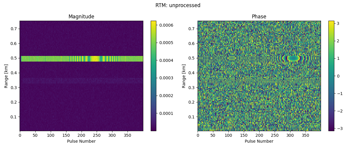
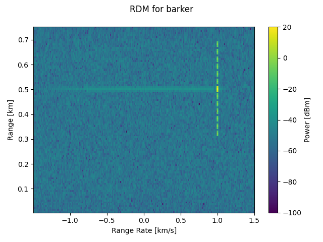
Minimal range-Doppler map example (used in the README).

Steps:

1. Define a radar system (carrier, power, gains, timing).
2. Choose a waveform (Barker-13 coded pulse).
3. Define a target (range, range-rate, RCS).
4. Generate the RDM — this builds the datacube, adds noise, applies the matched filter, and Doppler-processes to produce the range-Doppler map.

skin_snr.py

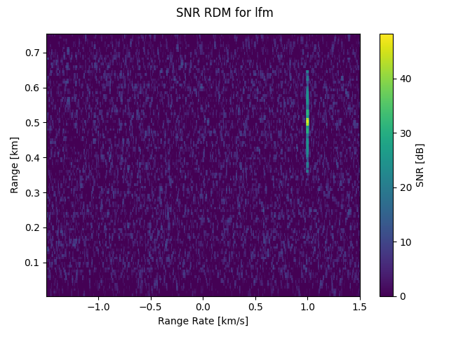
Skin return with SNR verification.

Generate an RDM for a single moving target using an LFM waveform, normalise to SNR voltage ratio with to_snr, and compare the measured peak SNR in the RDM to the range-equation prediction printed by check_expected_snr.

vbm.py

Velocity-Bin Masking (VBM) electronic attack example.

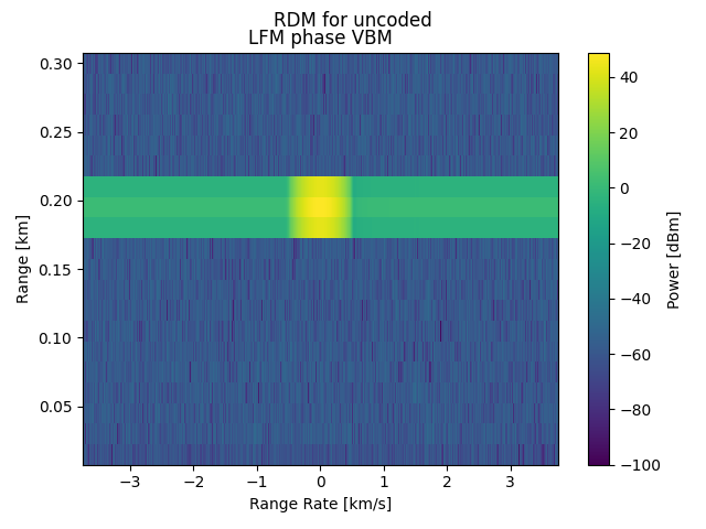
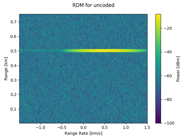
VBM is a DRFM jamming technique that spreads energy across multiple Doppler bins to mask the true target velocity. The jammer modulates the phase of the retransmitted signal in slow time, creating a band of Doppler noise centered on the target's Doppler cell.

Parameters:

• rdot_delta: width of the Doppler spread [m/s] — controls how many velocity bins are contaminated.
• rdot_offset: offset of the noise band center from the target [m/s].

The VBM noise appears as LFM in slow time. It is cleanest to observe when the target's range-rate is 0.

vbm_w_lfm.py

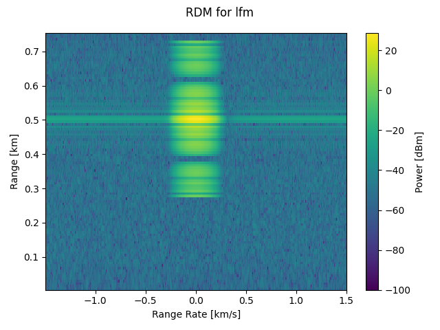
VBM electronic attack with an LFM waveform.

Same concept as vbm.py but using an LFM (chirp) waveform instead of uncoded. LFM provides better range resolution via pulse compression, so the VBM Doppler noise band is spread across fewer range bins but the same Doppler extent.

The target is stationary (range_rate=0) to isolate the VBM effect in the Doppler dimension.

SAR

spotlight_point_targets.py

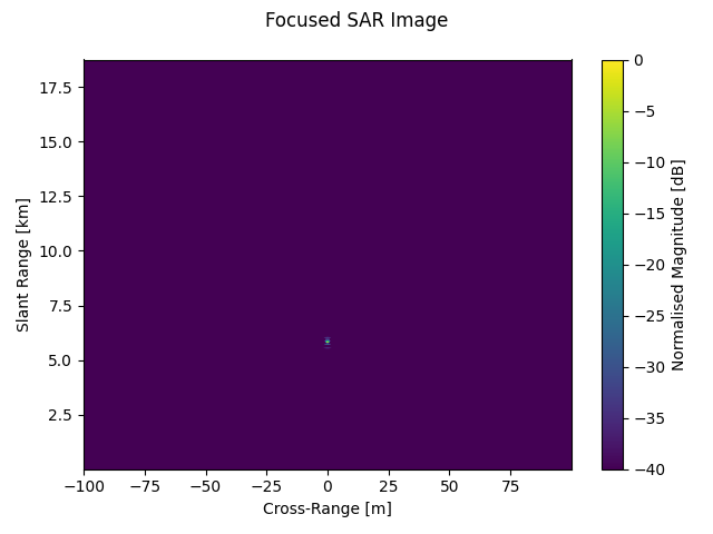
Spotlight SAR example: three point targets with beam-pattern weighting.

Demonstrates spotlight SAR by steering the antenna toward a scene centre and using a longer synthetic aperture than the stripmap example. The longer aperture yields finer cross-range resolution at the cost of a larger datacube.

Compared to stripmap_point_targets.py:

• aperture_length increased from 50 m to 200 m (4× more pulses)
• scene_center set to the middle target's position
• beamwidth set from a notional 0.5 m antenna: λ/D ≈ 0.06 rad

Cross-range resolution comparison (at ~5.8 km slant range):

Stripmap:  λR/(2L) = 0.03 × 5831 / (2 × 50)  ≈ 1.75 m
Spotlight: λR/(2L) = 0.03 × 5831 / (2 × 200) ≈ 0.44 m  (~4× finer)

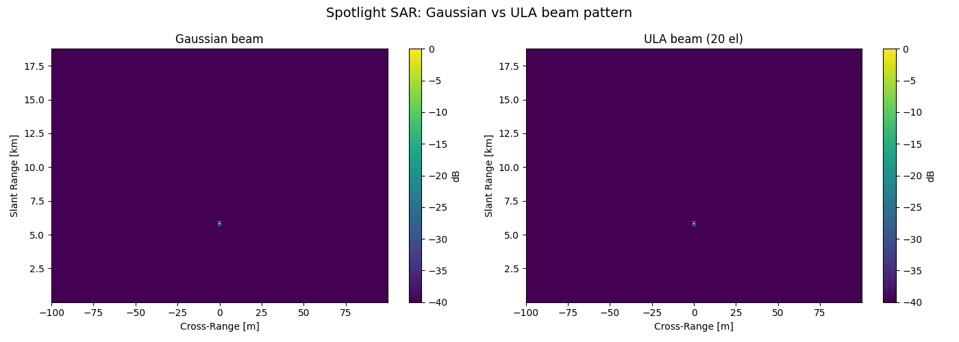
spotlight_ula_pattern.py

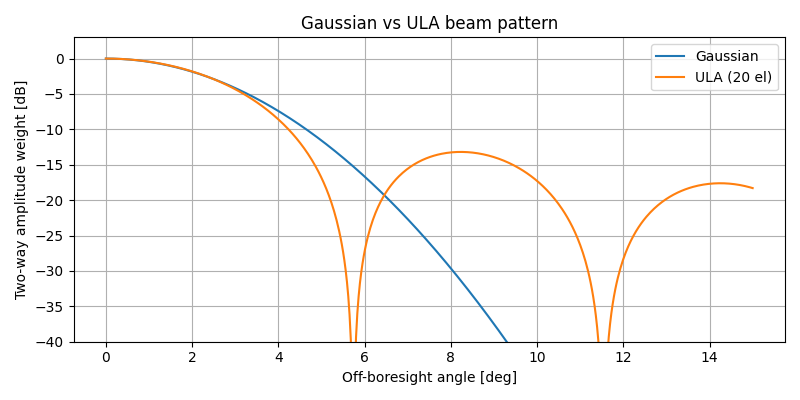
Spotlight SAR with a ULA-derived beam pattern.

Replaces the default Gaussian beam pattern with a realistic array factor computed from a 20-element uniform linear array (λ/2 spacing). The ULA pattern introduces sidelobes and nulls that affect how targets at different off-boresight angles are weighted.

Compares Gaussian vs ULA beam patterns by running the same scene twice.

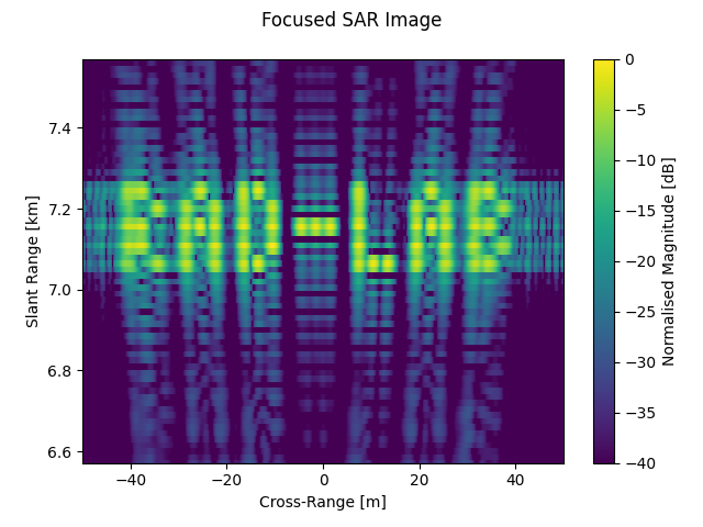
stripmap_point_cloud.py

Stripmap SAR point-cloud example: rendering "rad-lab" as text in a SAR image.

Demonstrates how a point cloud — many point scatterers arranged in a pattern — produces a recognizable shape in a focused SAR image. Each letter of "rad-lab" is defined on a 3×5 pixel grid, then mapped to physical target coordinates.

Parameter design summary:

• λ = 0.03 m (10 GHz carrier)
• Azimuth Nyquist: pulse_spacing = v/prf = 0.0125 m < λ/2 = 0.015 m
• Range resolution: c/(2*bw) = 30 m
• Cross-range resolution: λR/(2L) ≈ 1.06 m (at ~7 km slant range)
• Datacube: 1250 range bins × 8000 pulses
• aperture_length = 100 m (wider than default to fit 7 characters)
• Cross-range pixel pitch: 3 m (≫ 1.06 m resolution)
• Range pixel pitch: 60 m (2× the 30 m resolution)
• ~70 point targets total, all at z = 0, rcs = 10 m²

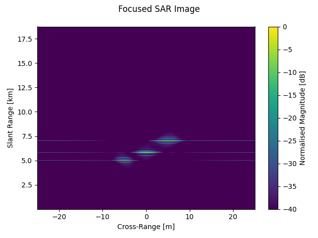
stripmap_point_targets.py

Stripmap SAR example: three point targets at different positions.

Demonstrates the basic SAR workflow:

1. Define SAR system parameters (SarRadar) and an LFM waveform.
2. Place point targets (SarTarget) in the scene.
3. Call sar.gen() to simulate the collection and focus the image.

The focused image should show three distinct peaks at the target positions. Cross-range resolution depends on the synthetic aperture length and range; range resolution depends on the waveform bandwidth.

Parameter design summary:

• λ = 0.03 m (10 GHz carrier)
• Azimuth Nyquist: pulse_spacing = v/prf = 0.0125 m < λ/2 = 0.015 m
• Range resolution: c/(2*bw) = 30 m
• Cross-range resolution: λR/(2L) ≈ 1.5–2.1 m (varies with slant range)
• Datacube: 1250 range bins × 4000 pulses
• Targets at slant ranges ~5.0, 5.8, 7.1 km (separated by ~800+ m, ≫ 30 m res) and along-track positions −5, 0, +5 m (separated by 5 m, > 1.5–2.1 m res)

Studies

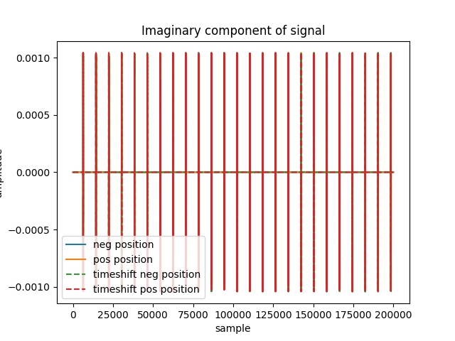
monopulse_considering_time_delay_between_elements.py

Study: does the inter-element time delay matter for monopulse?

In a phased array, each element receives the signal at a slightly different time due to the wavefront arrival angle. The standard monopulse model only applies the carrier-frequency phase shift (exp(j2pidsin(theta)/lambda_c)), ignoring the baseband time delay.

This study compares two approaches:

1. Phase-shift only (standard): multiply each element's datacube by the steering vector phase at the carrier frequency.
2. Phase-shift + time delay: also apply the true time delay to the baseband signal, which shifts the waveform samples.

Findings:

• When fcar >> bw, the time delay is negligible (lambda/2 at the carrier is lambda/100 at IF frequencies — very little phase change).
• Regardless of fcar, the monopulse angle estimate is barely affected.
• The study uses fcar=1 GHz with bw=200 MHz (ratio=5) to stress-test this.

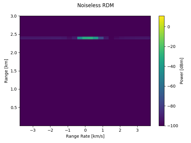
vbm_methods.py

Compare VBM noise generation methods.

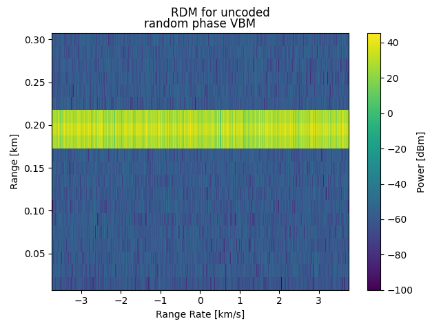
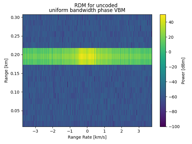
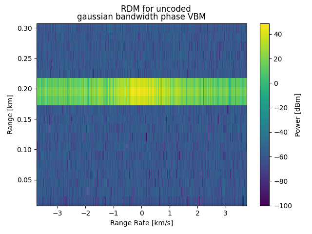
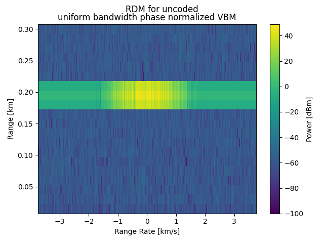
The VBM (Velocity-Bin Masking) jammer spreads energy across Doppler bins by modulating the retransmitted signal's phase in slow time. There are several ways to generate that phase modulation, listed here from simplest to most physically accurate:

1. random_phase: each pulse gets an independent random phase — produces flat Doppler noise but doesn't respect the prescribed bandwidth.
2. uniform_bandwidth_phase: random phase filtered to a uniform spectral shape within the target bandwidth.
3. gaussian_bandwidth_phase: random phase filtered to a Gaussian spectral shape — more realistic but doesn't match the prescribed width exactly.
4. gaussian_bandwidth_phase_normalized: same as (3) but normalized.
5. lfm_phase: slow-time LFM chirp — the only method that precisely matches the prescribed rdot_delta bandwidth.

Each method generates an RDM so you can visually compare the Doppler spread.